We proudly present the first part of our Turkish subword manifesto: how Turkish language modeling benefits from morphology. In this article, we compare character-, word-, and morphology-aware subword tokenization, where subwords are created by following the language’s natural morphological structure. Unsurprisingly, the best results come from morphology-aligned subwords. Character-level models are competitive, while word-level vocabularies perform poorly. Let’s dive into Turkish subwords together.
Turkish is an agglutinative language: new words are formed by attaching multiple suffixes to a root. This structure is both elegant and powerful, but it also challenges “vanilla” tokenization approaches. To model Turkish effectively, we must design vocabularies around its true building blocks—morphological units—rather than whole words alone.
Our recent work, “Optimal Turkish Subword Strategies at Scale: Systematic Evaluation of Data–Vocabulary–Morphology Interplay,” offers a principled way to dissect Turkish into tokens and to build optimal vocabularies. We examine two broad eras:
- Pre-transformer tokenization approaches
- Transformer-era tokenization with WordPiece-style vocabularies
This post focuses on the pre-transformer era. If you’re interested in WordPiece + Turkish, see Part 2 of the blog. We proceed from lower to higher compute: character-level and word-level vocabularies, then morphology-aware subword vocabularies.
We evaluate across three tracks: our new TrGLUE benchmark, Named Entity Recognition (NER), and POS–Dependency–Morphology tagging on a treebank.
- TrGLUE tasks selected: CoLA (acceptability - Matthews Correlation Coefficient), MRPC (semantic equivalence - accuracy), MNLI (entailment - accuracy), SST-2 (sentiment analysis - accuracy), and STS-B (semantic similarity - Pearson correlation coefficient).
- NER: WikiNER (Turkish) i, evlauated with F1 over entity spans.
- Treebank: BOUN treebank for POS, dependency, and morphological tagging; all evaluated with token based accuracy roughly.
In this post we’ll focus on TrGLUE and POS-Dep-Morph tasks to reveal subword power in the most distinguished way.
To ground the discussion, consider how different vocabularies segment the Turkish word “gittim” (“I went”):
- Character-level:
g #i #t #t #i #m - Word-level:
gittim - Morphology-aware subwords:
git #ti #m
Character-level offers maximal granularity but long sequences; word-level is compact yet brittle to inflection; morphology-aligned subwords strike a balance by respecting the language’s productive suffixation.
Modelling
To isolate vocabulary effects, we kept architectures comparable across setups.
TrGLUE tasks:
- Char-level: CNN encoder over character embeddings (no external pretraining).
- Word/subword: BiLSTM over embeddings initialized with Google word2vec; embeddings remain trainable.
NER:
- BiLSTM with a token-classification head.
- Word-level prediction per word: direct word token or pooled subword/char states.
- Subwords: only the first subword receives B-/I- tags; others are masked/forced O.
- Characters: BIO per character; contiguous spans merged back to words for F1.
POS–Dep–Morph:
- Joint multi-task over a shared BiLSTM.
- UPOS: linear head. Dependencies: deep-biaffine arcs/relations. Morphology: per-attribute classifiers (incl. NONE).
- For subword/char inputs, word representations are pooled or composed; all predictions/evaluation stay at the word level.
Character-level vocab
Character-level vocabularies are easy to keep and generate, one keeps only a set of characters as the vocab items, usually a list of letters, digits and some signs. Some keeps punctuation marks, some don’t. In our work, we made a capital aware vocabulary, keps capital letters, lower letters, digits and non-sentence punctuation. We cleaned sentence level punctuation such as periods, commas and semicolumns.
Despite their simplicity, character-level models hold up surprisingly well on several fronts. They excel when tasks are driven by surface cues and morphotactics, and they provide a strong tokenizer-free baseline that’s robust to OOV forms, typos, and tokenization noise. Where they fall short is in tasks that demand longer-range composition and precise lexical semantics.
Surprisingly, TrGLUE performance is not bad at all. We can summarize the TrGLUE success as follows:
- Strong on surface sentiment: SST-2 lands around 84% accuracy—polarity and intensifiers are well captured by local character n-grams.
- Serviceable on inference: MNLI reaches ~67%—morphology signals help, but lack of longer context caps performance.
- Weak on fine-grained structure/semantics: CoLA (MCC ~0.08) and STS-B (ρ ~0.12) remain challenging due to limited compositional depth and lexical grounding. Paraphrase (MRPC) sits in the middle at ~62% accuracy.
Coming to NER task, char-level vocab
- delivers an F1 around 0.70 with pure character inputs—no explicit tokenization needed.
- is strong with suffix patterns, orthographic regularities, and consistent morphotactics help recover spans.
- hiccups at boundary drift at span edges; confusions among close types (e.g., organization vs. location).
POS–Dep–Morph success is whole another story.
- POS accuracy ~91.6 and morphology micro-accuracy ~96.2, with uniformly high scores across attributes (e.g., Tense, Mood, Voice, Case).
- Dependency parsing is the pinch point: UAS/LAS ~65/57, reflecting difficulty with long-distance attachments without strong token-level context.
Character-level models trade syntactic attachment quality for morphological fidelity. Against BERTurk on the same treebank, token-based models achieve much higher UAS/LAS and slightly better POS, but trail dramatically on morphology. This contrast highlights complementary inductive biases: characters capture affixal and orthographic signals extremely well; pretrained token encoders better model head–dependent structure and broader semantics.
What to take away
- Robust baseline: Character-level modeling is a clean floor for evaluation—gains from subwords can be attributed to segmentation and lexicalization rather than preprocessing.
- Strengths: Excellent morphological fidelity; competitive on surface-driven classification; resilient to OOVs and noisy text.
- Limits: Struggles with grammatical acceptability, graded similarity, and long-distance syntax—areas where morphology-aligned subwords and stronger contextual modeling help.
- When to use: Particularly attractive in agglutinative, low-resource, or noisy settings where vocabulary explosion and tokenization errors are costly.
Stepping up from characters to whole words trims sequence length, but what happens in downstream task success? We find out next.
Word-level vocab
From one extreme to the other, now we keep all vocab words as they’re, no way of decomposing further. Again we kept all words with their casing, we used cased-vocabs in our work . We cleaned all sentence punctuation as well.
Here, we first need to adapt some notation. Let V denote the full word vocabulary extracted from training and sorted by frequency, and let K be the size of the retained prefix (top-K types). Here is a quick example, let’s say these are all the sorted corpus words by frequency:
ben 500
de  500
.
.
.
gelmemezlikten 1
and let’s again assume we have 500 unique entries in the vocab and total of 10K words. Here if we take K=2, top-2 words will cover 10% of all corpus words. As a result the sentence Oraya ben de gittim will tokenize as <UNK> ben de <UNK>.
As a result we define 3 notions:
- training coverage: the fraction of training tokens accounted for by the top-K types;
- test coverage: the fraction of test tokens covered by the same top-K types learned from training;
- the relationship between coverage (or K) and final task scores.
As one can imagine, per task first we created corpus words and count files, then make coverage calculations, finally created vocab files that correpond to the coverage percentages. One can see the code for vocab creation under the project Github repo and some example vocab files under the same repo.
Let’s quickly go into the tasks and see what is net effect of choosing top-K words to form our vocabs.
TrGLUE tasks
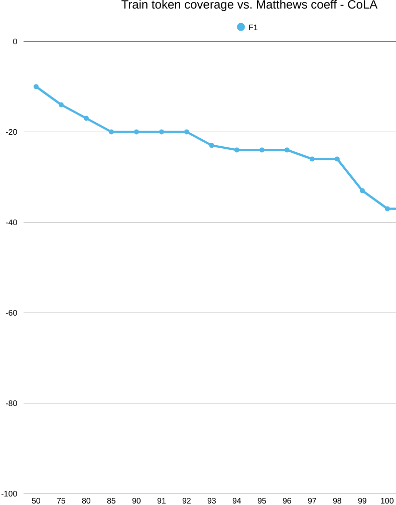
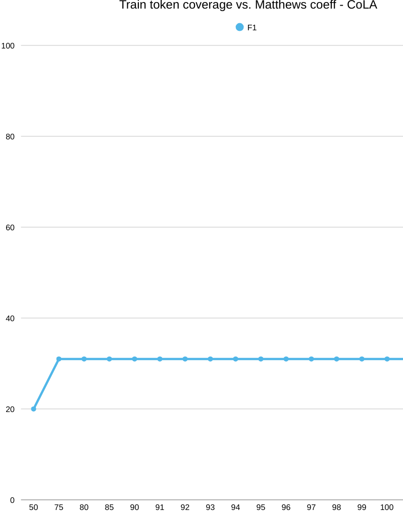
First we have a glance at CoLA’s coverage and success-coverage graphics, together with explainability of an example sentence. On CoLA, cranking up word coverage doesn’t help. Even as we keep more words, the model’s MCC stays below chance (0 MCC means random guess) and actually slips downward. The issue isn’t “do we have the words?”—it’s “what do those words let the model represent?” A big, sparse word list can’t capture the grammar signals CoLA cares about (long-distance rules, subcategorization, function words in context). As we add more entries, we mostly add rare, morphologically busy variants, which spreads the data thin and nudges the model to memorize surface quirks instead of learning structure.
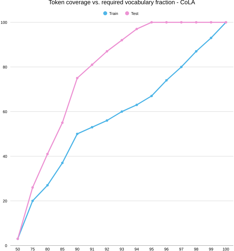
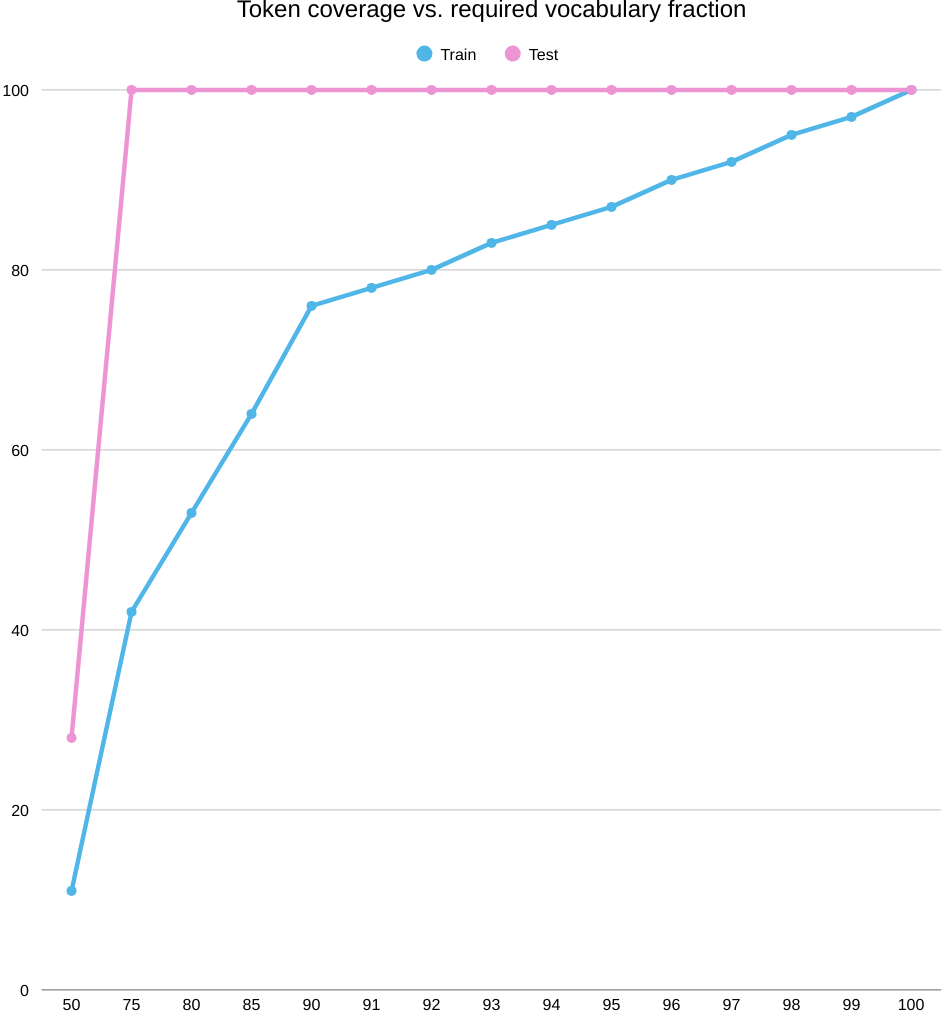
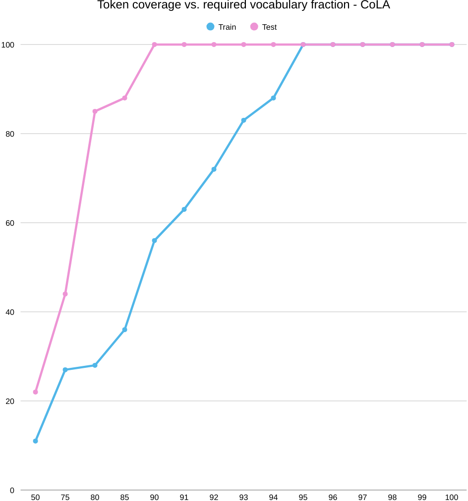
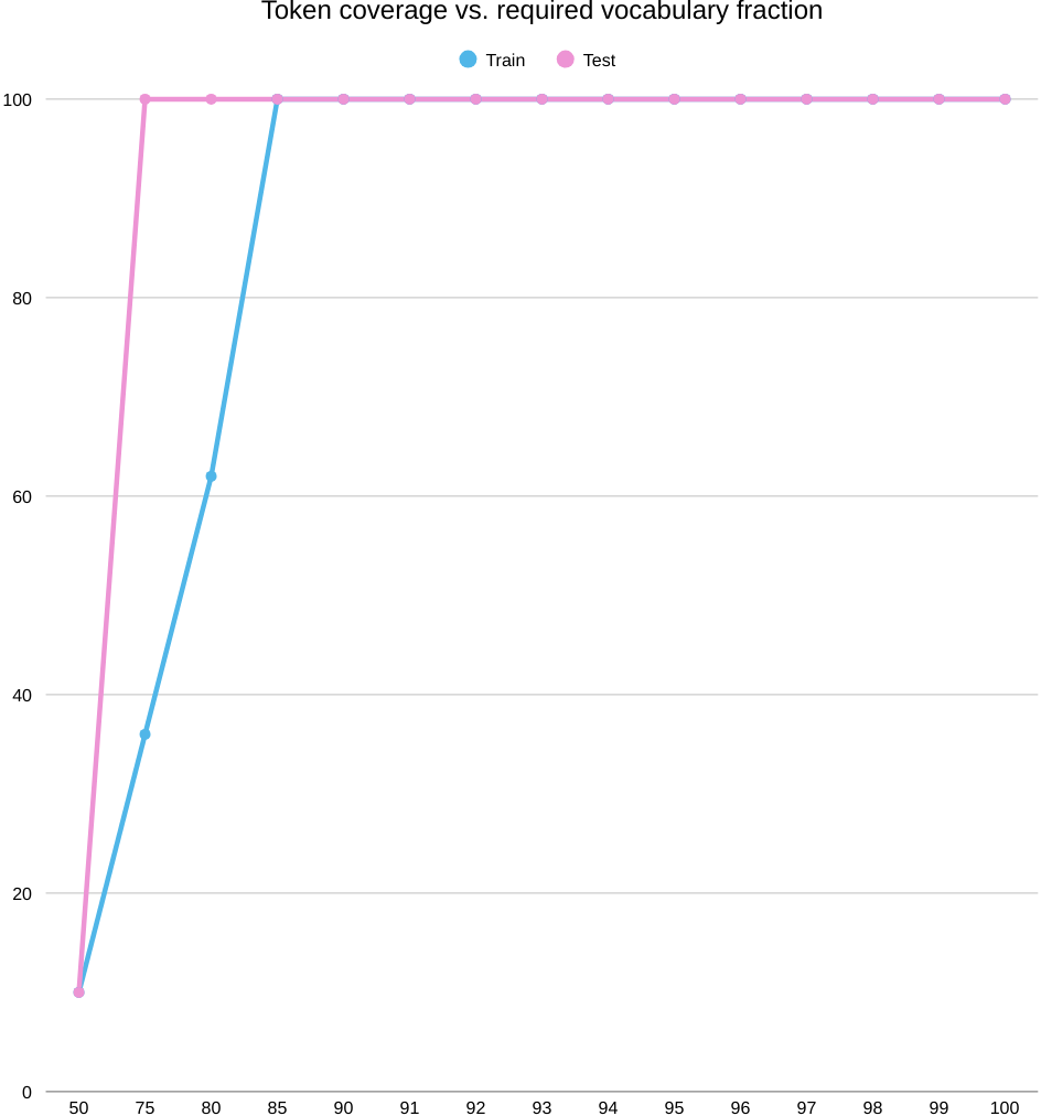
First, the coverage plot: as you keep more of the word list (move right on K/|V|), test coverage shoots up quickly and flattens around the mid‑90% range, while train coverage climbs more slowly. Translation: plenty of tokens seen in training don’t transfer cleanly to the test set, so you need to keep a large chunk of the vocabulary just to cover train, even though test looks “covered” much earlier.
Now the success plot: when we line up train token coverage against CoLA score (MCC), every point is below zero—and the curve gently slides downward as coverage grows. Rough numbers: around −10 MCC at 50% coverage and drifting to about −36 at full coverage. So, even with near‑complete coverage, the word‑level model still can’t judge acceptability well; the roadblock is representation, not how many words we keep.
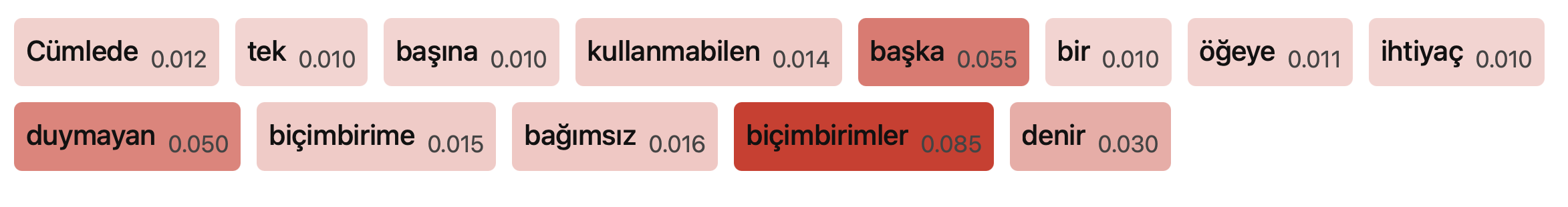
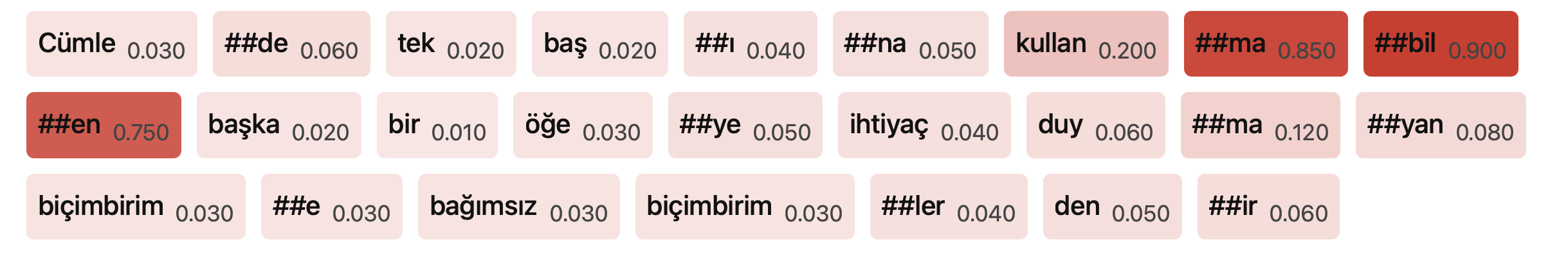
Finally, the explainability view (top‑80% vocab): the attributions are faint and blurry: out‑of‑vocabulary items barely register, and even forms like biçimbirime/biçimbirimler only get mild highlights. There’s no crisp morphosyntactic pattern—another hint that this setup is leaning on surface frequency and label priors rather than the grammatical cues CoLA requires.
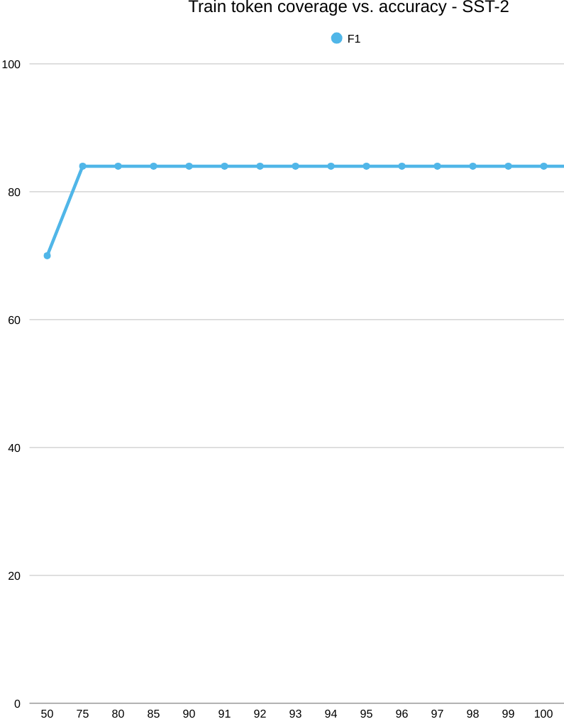
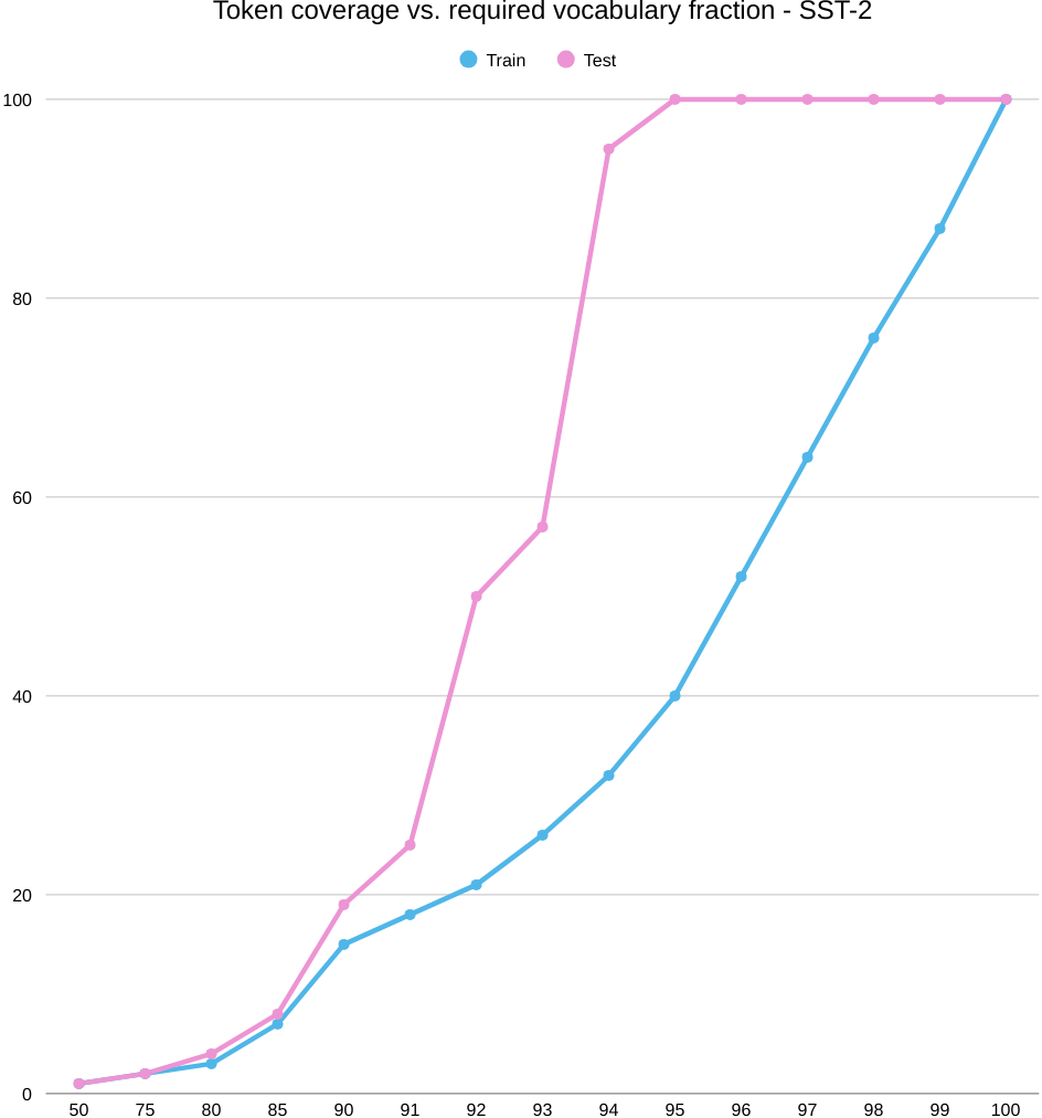
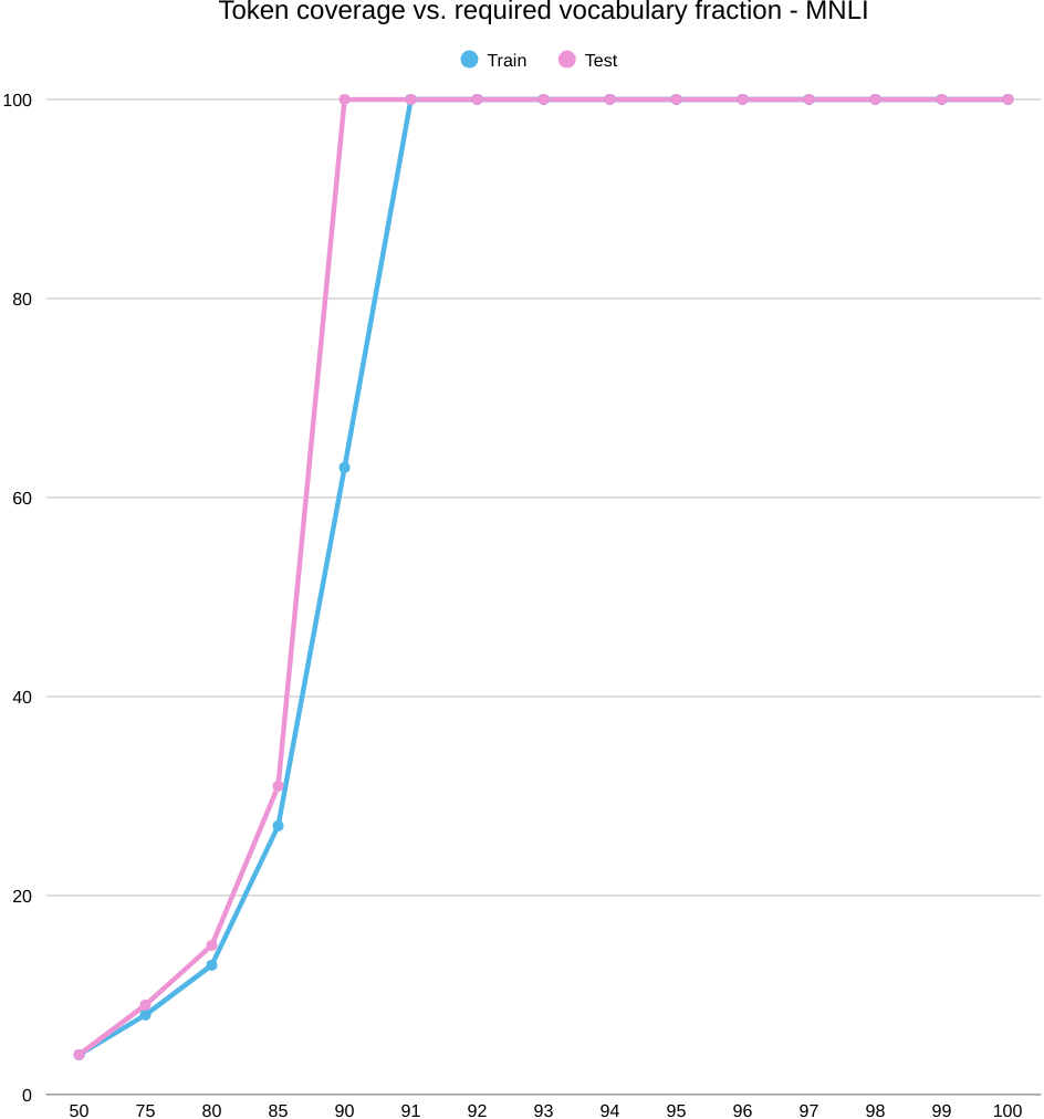
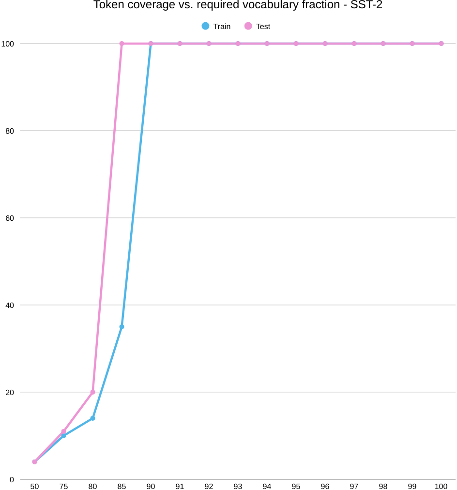
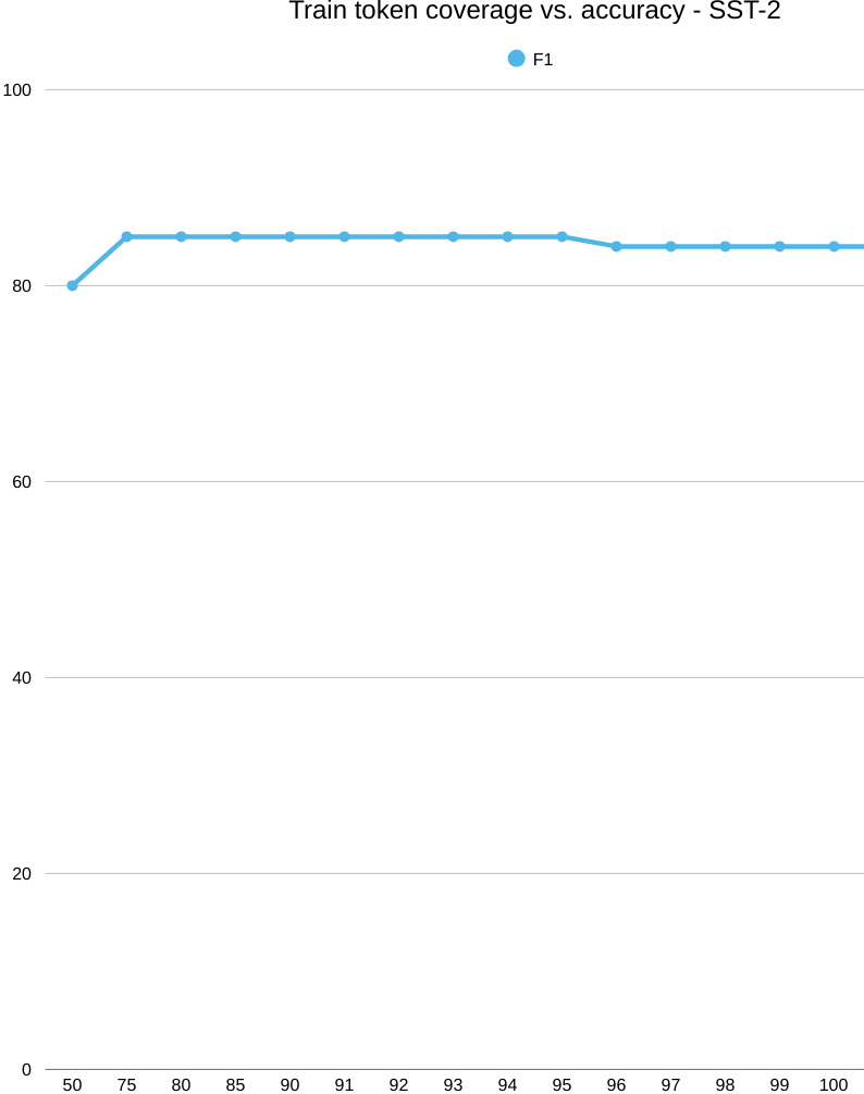
Next comes, SST-2, a completely different picture. In the below picture, we start with coverage. As you keep more of the word list (increase K/|V|), test coverage spikes quickly and levels off around 93–95%, while train coverage climbs more slowly. So the test set “looks covered” with a relatively small vocabulary, even though train still needs a larger slice to catch up.
Now the accuracy curve. Performance jumps early—about 69% accuracy at 50% train coverage up to roughly 85% by the 75–80% mark—and then it plateaus. Past that elbow, adding rarer words doesn’t help: the model already has the key sentiment cues it needs. Think frequent polarity markers and phrases like “hiç,” “çok kötü,” “berbat,” “beğenmedim” on the negative side, and “mükemmel,” “harika,” “bayıldım” on the positive side. In other words, sentiment at the word level is powered by a compact lexicon of strong signals; once those are in, more tail types add little.
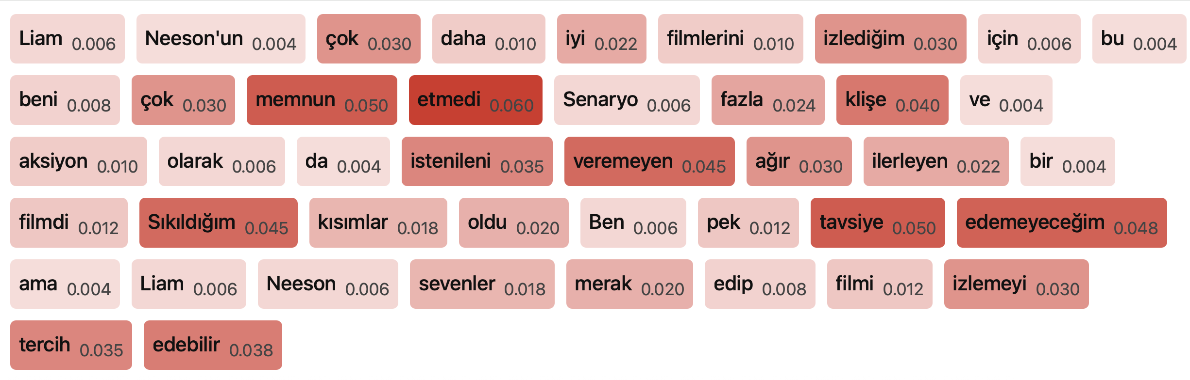
Looking at the explainability snapshot (top-80% vocab), attributions cluster on sentiment-bearing words and predicate cues: “memnun etmedi,” “klişe,” “ağır,” “Sıkıldığım,” “tavsiye edemeyeceğim,” and “tercih/edebilir.” This matches the plateau story—the model keys off a small set of high-impact tokens. This model didn’t model morphology, but it didn’t need to anyway, distinguishing some sentiment indicating phrases were totally enough.
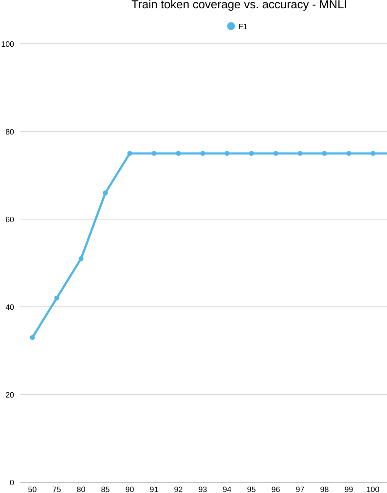
Across MNLI, MRPC, and STS-B, test coverage saturates earlier than train, and performance shows an early elbow followed by a plateau: MNLI hovers around 0.70 accuracy, MRPC around 0.60, and STS-B around 0.25 (Pearson/Spearman). In contrast, SST-2 reaches its ceiling once a compact polarity lexicon is included. Overall, expanding word-level coverage doesn’t improve generalization on the non-sentiment tasks, pointing to the need for richer contextual representations.
POS-Dep-Morph
Shifting from TRGLUE’s sentence-level tasks to token-level POS-Dep-Morph changes the game: instead of judging sentence meaning or acceptability, the model has to label words and their relations, often relying on fine-grained morphology and syntax. In this setting, simple word-level vocabularies might look appealing at first glance—high-frequency function words and common inflected forms quickly boost coverage—but the underlying demands are different: accurate POS tags, dependency arcs, and morphological features hinge on context-sensitive cues that a surface word list can’t encode.
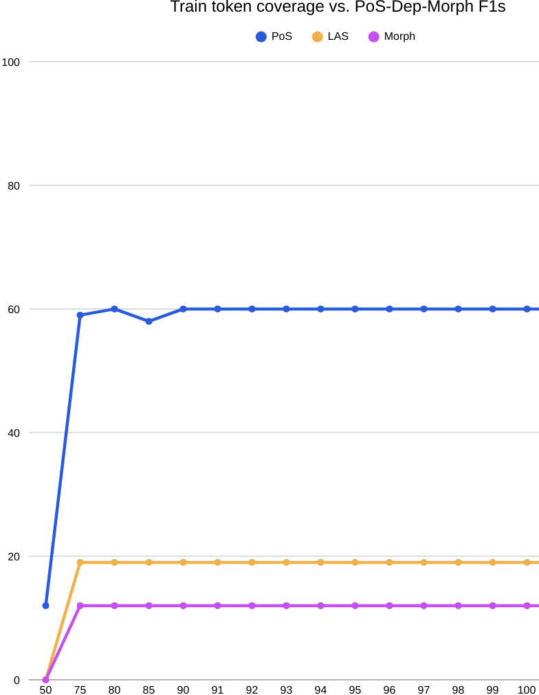
Let’s move onto the solid numbers in the below figure. The success curves flatten hard after roughly 75% train coverage: keeping more of the word list does not lift POS, LAS, or Morph F1, which stall near ≈60/19/12—far below character-level baselines (≈91/65/96). This isn’t a coverage problem; it’s a representation problem. In BOUN’s morphology-heavy setting, rich inflection splits lemmas into many sparse surface types, creating a long tail that a word inventory can’t generalize over. The coverage plots underscore a train–test mismatch, too: token mass accumulated on train doesn’t reflect what’s needed at test time. Practically, this argues against word-level vocabularies for POS-Dep-Morph on BOUN: character or subword models, ideally with explicit morphological supervision, are required to capture inflectional variation and reach competitive accuracy.
On BOUN, coverage accumulates unevenly across splits: as K/|V| grows, train token coverage rises only gradually, while test follows a different trajectory, signaling a mismatch between the ranked word list and the test distribution. Mapping train coverage to performance, POS, LAS, and Morph F1 all plateau by roughly 75% coverage—around 60, 19, and 12 respectively—and stay flat thereafter, showing that retaining larger fractions of the word list doesn’t yield gains. The explainability view reinforces this: at top-80% vocab, attributions cluster on in-vocab function words (“Bir,” “yandan,” “da”) while OOV content words receive flat, low weights, revealing limited morphological awareness. Altogether, the curves and saliency patterns point to distribution shift and the inefficiency of word-level vocabularies on this morphologically rich dataset: higher token coverage demands large K yet fails to improve POS, dependency, or morphology performance. This is all expected, there is no way a pure word vocab can comprehend moprhemes of Turkish. This is all expected, there is no way a pure word vocab can comprehend morphemes of Turkish.
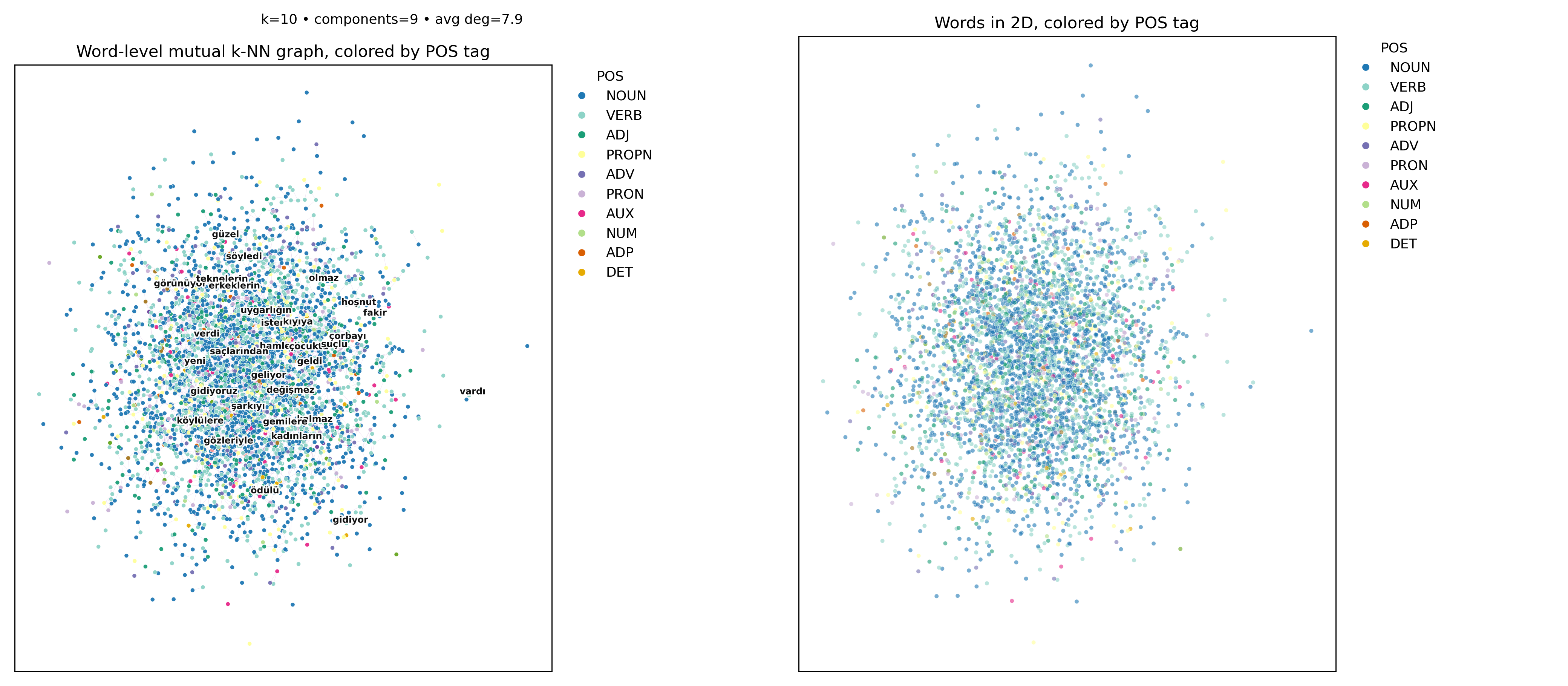
Going one more step further and looking at the word embeddings figure (the very first figure up this page), the embeddings set up the core limitation that our analyses will unpack: in the 2D projections, POS colors are thoroughly intermingled and the mutual k-NN graph links cut across categories. In other words, whole-word embeddings fail to organize Turkish by syntactic role. This is not a coverage artifact—the plots aggregate thousands of tokens—but a representation issue: rich inflection explodes surface forms, so a word-level space mostly groups by frequency and topical co-occurrence rather than by morphology or part of speech. The visual takeaway is simple and intentional: at the word level, Turkish syntax does not “fall out” of the geometry.
Morpho-subwords
Now comes our rock-star section, morpho-subwords of Turkish. For this part, we needed some more data preparation steps. Before all, let’s start easy and see how coverage works. Say this is our vcorpus words:
gitmedim
gitmemek
gitmek
gittim
geldim
gelmedim
gelmemek
gelmek
bittim
bitmedim
bitmek
bitmemek
ghostluyorum
.
.
.
Then we decompose all the words and sorted the resulting morphs by frequency, let’s say this is the result:
##mek
##me
##di
##ti
##uyor
##m
##um
git
gel
bit
.
.
.
If we take K=1 , ##me alone won’t cover any vocab words. However if we take K=8, it’ll cover the words gitmek, gitmemek, gitmedim, gittim. With K=9 we move onto the next lemma gel and cover 4 more words. Continuing in this fashion, we can advance K a bit, that might result in covering quite many vocab words.
Coming to the practical side, we decomposed words into moprhemes by Turkish morphological tooks including Turkish spaCy models and Zeyrek. Decomposing words take some time, hence we created cache files of word decompositions, like this example. This way we the morpho-tokenizer can look up word decompositions during training time as well as in the coverage calculations. The coverage calculator is similar to word-level’s, but this time we cover with subwords. After vocab work, we are ready to explore modelling results in the next subsection.
TrGLUE results
Coming to TrGLUE results, the picture is quite different than word-level results. The below figure explains task success vs task coverage for CoLA, MNLI and SST-2:
Across CoLA, MNLI, and SST‑2, morphology‑aware subwords punch way above their weight. The coverage curves climb fast—almost vertical for MNLI and SST‑2—and with only a small slice of the morpheme inventory we’re already brushing up against full train/test coverage. In plain terms, a compact set of productive stems and suffixes explains most of the tokens that actually show up. That’s the big advantage over word‑level tokenization: to get similar coverage with full words you need a much larger lexicon, and you still get dinged by derivations and inflections that spill into OOV territory. The morph inventory stays small, coverage saturates, and you don’t pay the vocabulary‑bloat tax.
Performance mirrors this story. As we add morphemes in order of coverage, MNLI and SST‑2 level off quickly—the core set buys you most of the gains, and after that it’s diminishing returns. CoLA is steadier and a little flatter, which makes sense for a task that’s sensitive to agreement and case rather than raw lexical variety. The task‑specific intuition checks out: in SST‑2, polarity often hinges on a few markers like -ma/-me, so it saturates early; in MNLI, getting negation, modality, and case markers right stabilizes contradiction vs. neutral decisions; and in CoLA, person/number/case morphology helps localize acceptability issues, so progress is slower but consistent.
Zooming out, the takeaway is simple: compared to word‑level tokenization, morphology‑aware subwords deliver near‑complete coverage with a fraction of the vocabulary, cut down OOV‑driven variance, and hit comparable or better accuracy. It’s a cleaner efficiency–performance trade‑off for Turkish. The same pattern shows up on STS‑B and MRPC, too—fast coverage saturation, early performance plateaus—with our morph‑subword BiLSTM landing around 0.45 on STS‑B and 0.62 on MRPC. Morphology smooths out lexical variation; what’s left on the table is mostly semantics and pretraining scale.
With coverage and downstream trends in place, we next ask what the model is actually using: the explainability analyses below trace decisions back to specific morphemes, showing which stems and affixes drive predictions and how their importance shifts across tasks.
 (a) Morph-level attributions on sample CoLA sentence | 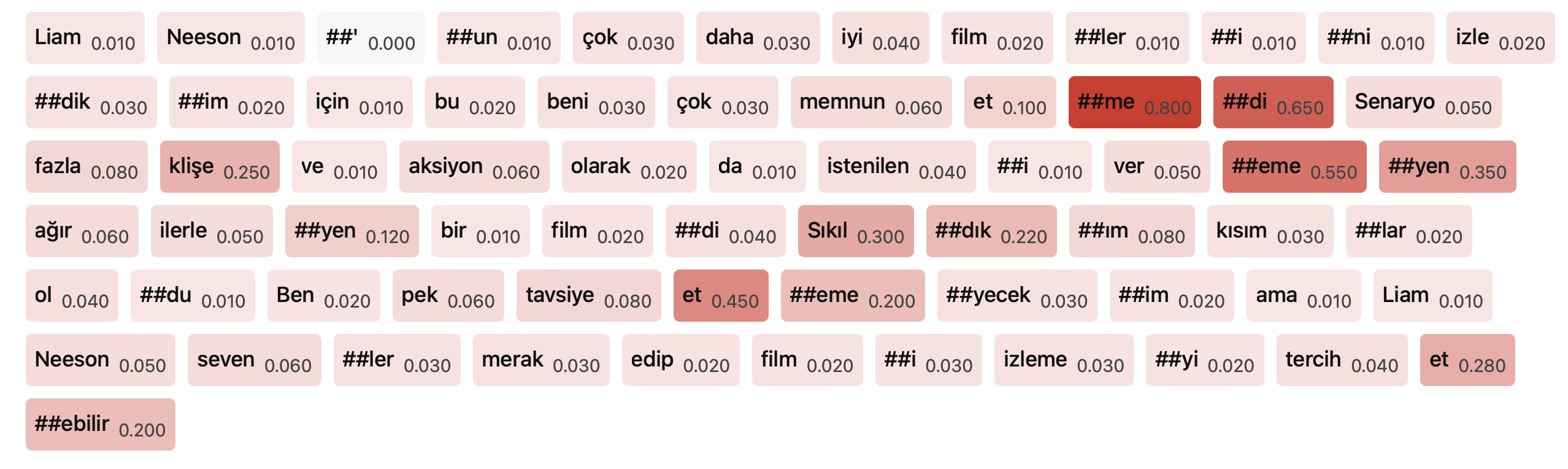 Morph-level attributions on sample SST-2 sentence |
Figure above shows the same story from the inside. In both TrGLUE examples, the strongest positive attribution lands on morphologically salient pieces that actually move the label: negation morphemes, derivational markers that flip part‑of‑speech, and clause‑level connectives. Low‑content function words stay quiet. We also see complementary evidence: stems carry the broad semantics, while suffixes nudge the decision—polarity, modality, entailment—over the line. In other words, the model is composing meaning from morph‑subwords rather than keying on whole‑word surface forms.
Building on that, the next section zooms out from task labels to token‑level structure, where suffixes really shine: we’ll see how morph‑subwords line up with POS tags, dependency edges, and fine‑grained morphological features—and how those suffix cues consistently carry the heaviest lift.
POS-Dep-Morph
So far we’ve looked at coverage, accuracy, and why the model’s attributions cluster on meaningful morphemes. Now we turn to the token‑level scaffolding of Turkish: parts of speech, dependency arcs, and morphological features. This section asks a simple question with big consequences—how well do morph‑subwords align with the linguistic signals that syntax and morphology annotate? We’ll show that stems anchor broad semantics, but suffixes are the precision tools: they encode agreement, case, tense/aspect/modality, and clause structure, and they light up exactly where POS and dependency decisions hinge.

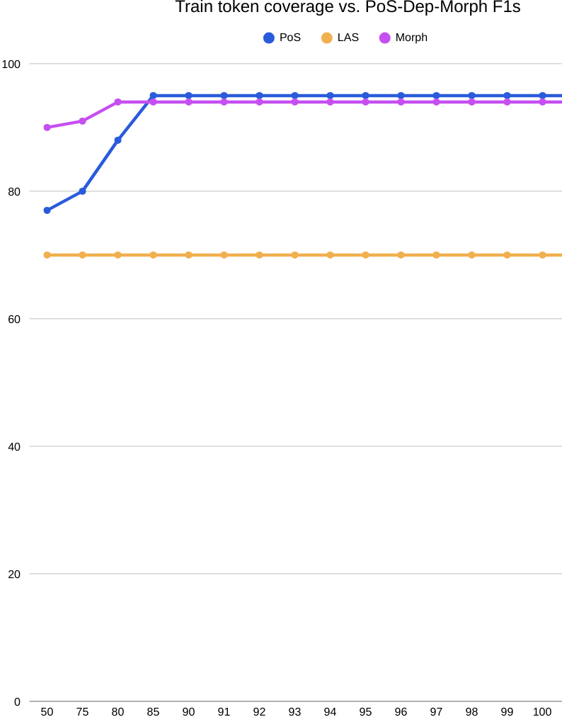
Looking at the figure above, as coverage increases, the morph‑subword models improve quickly and then settle. POS and Morph F1 rise steeply from low coverage and flatten around the 80–85% mark, essentially reaching their ceilings. LAS is flatter overall once the basics are in place: as soon as the key case and possessive cues are retained, head selection stabilizes and extra vocabulary buys little. What’s striking is how compact the inventory can be while doing this. On the test split, you’re near full coverage with roughly three‑quarters of the morpheme set; the train split tops out at about 83–85%. That efficiency is exactly what we don’t get with word‑level tokenization, which needs a much larger lexicon to approach the same scores and still struggles with OOVs.
Looking inside the attributions clarifies why the curves behave this way. The model consistently leans on inflectional endings—number, case, tense/aspect—more than on stems, especially for nouns and verbs whose bases are ambiguous. Suffixes like -ler (plural), -de/-da (locative), -yor (progressive), and -du (past) dominate the signal that determines POS and supports dependency decisions. Stems set the broad semantics, but these endings are the precision tools that disambiguate category and structure, which is why performance plateaus once those high‑value morphemes are included.
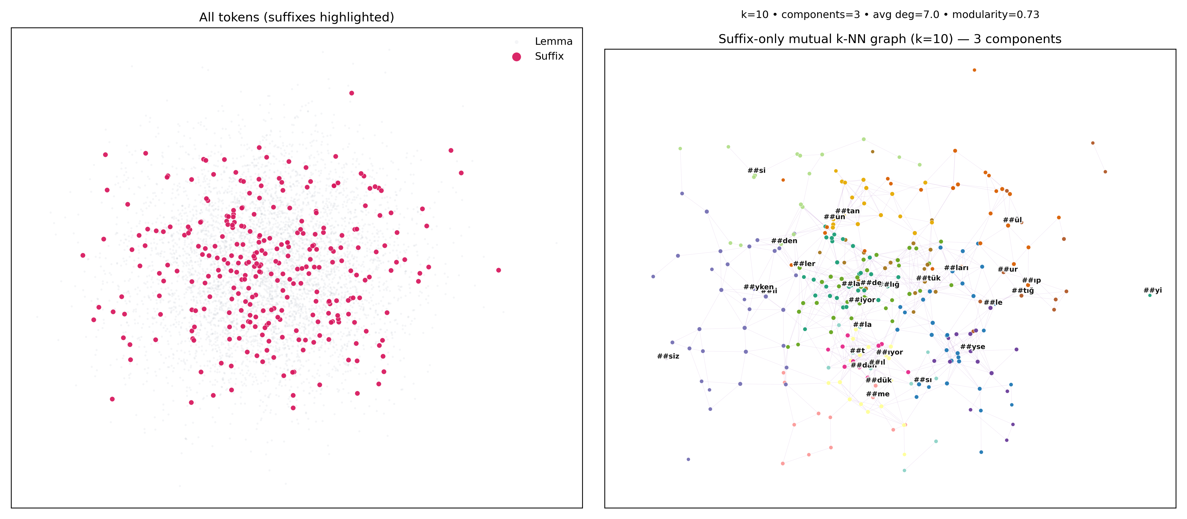
Having just shown which morphemes drive decisions, the subword embedding plots illustrate why: when tokens are morphology-aware, neighborhoods are shaped by stems and productive suffixes. You see tighter local structure, clearer POS tendencies, and clusters that reflect case, negation, person/number, and derivation. Even without pretraining, these subword embeddings compress the vocabulary, reduce OOV churn, and align geometry with grammatical cues. The figures reinforce the story from attributions: stems carry semantics; affixes steer syntactic and polarity decisions—so the embedding space becomes more interpretable and compositional.
Once again putting the embedding plots side by side, the contrast is stark. Word-level spaces blur categories and require huge lexicons for mediocre structure; morphology-aligned subwords achieve near-complete coverage with a compact inventory and yield neighborhoods that respect Turkish morphotactics. Practically, this means better generalization with fewer tokens, more stable behavior on inflected variants, and clearer saliency maps. For Turkish—and other agglutinative languages—the figures make the case: if you want embeddings that reflect syntax and morphology, don’t stop at whole words; build the vocabulary around the morphemes the language actually uses.
Resources
Here are your readings if you wanna explore the topic further:
Research paper
Preprint available at Arxiv.
Github
Github repo for all the related computations: Github for subwords
Second part of the blog
is dedicated to how Turkish vocabs interact with WordPiece tokenizer. The post is on Medium.
Hugging Face
We host WordPiece tokenizers and corresponding BERT models in our HF repo: Turkish NLP suite HF repo.
Special Thanks
goes to Google Cloud TPU program as always, where we made all the Transformer training; without them this work wouldn’t be possible at all